Analytic Bayesian Inference
For our simple model, an exact analytical solution to the Bayesian linear regression problem is possible. It is described in detail in the Wikipedia entry on Bayesian Linear regression. We will thus refrain from explaining every mathematical detail on focus on the main steps and results. Please note that such a solution is only possible in a handful of simple models and the vast majority of models encountered in practice require approximation.
Recap
During the following calculations, we will be relying heavily on the knowledge about the Normal and Gamma PDFs, so here is a quick recap. The Normal distribution is defined as follows:
\[\mathcal{N}(w|\mu,\tau^{-1})=\sqrt\frac{\tau}{2\pi}\exp\left[-\frac{\tau}{2}(w-\mu)^2\right]\]The mean is $\mu$ and the precision (inverse of the variance) is $\tau$. Its natural logarithm is as follows:
\[\log \mathcal{N}(w|\mu,\tau^{-1})=\dfrac{1}{2} \log\dfrac{\tau}{2\pi}+\left[-\frac{\tau}{2}(w-\mu)^2\right]\]For the Gamma distribution we have:
\[\log \mathcal{Ga}(\beta|a,b)=\frac{b^a}{\Gamma(a)}\beta^{a-1}\exp(-\beta b),\]with shape and rate parameters $a$ and $b$, respectively. The mean of the Gamma PDF is $a/b$ and the variance is $a/b^2$. Its natural logarithm is as follows:
\[\mathcal{Ga}(\beta|a,b)=a\log b - \log \Gamma(a) + (a-1)\log \beta-\beta b\]The Likelihood function
As mentioned before the likelihood function $L(\mathcal{D}|w,\beta)$ describes the likelihood of observing the data $\mathcal{D}$ given the unknown parameters $w$ and $\beta$ according to our linear regression model. Since the measurement error follows a Normal distribution with zero mean, the probability of observing a single data point (pair of $x$ and $y$) can be expressed as:
\[p(y|x,w,\beta) = \mathcal{N}(y|wf(x),\beta^{-1})\]In words, we expect our model output $y$ to be normally distributed with a mean at the model-predicted value $wf(x)$ and a precision of $\beta$. If we now have a dataset $\mathcal{D}$ of $N$ data points, which are independent from each other (this is an important detail of the model assumptions), we can simply multiply the individual probabilities to arrive at the overall likelihood
\[L(\mathcal{D}|w,\beta) = \prod_{i=1}^{N} \mathcal{N}(y_i|wf(x_i),\beta^{-1})=\left(\frac{\beta}{2\pi}\right)^{\frac{N}{2}}\exp\left[-\frac{\beta}{2}\sum_{i=1}^{N}(y_i-wf(x_i))^2\right]\]Switching to vector notation where we define $x=(x_1,x_2,…,x_N)^T$ and $y=(y_1,y_2,…,y_N)^T$, i.e. both vectors have a single column, we can simplify the likelihood as follows:
\[L(\mathcal{D}|w,\beta) = \left(\frac{\beta}{2\pi}\right)^{\frac{N}{2}}\exp\left[-\frac{\beta}{2}\left(y^Ty-2y^Tf(x)w+f(x)^Tf(x)w^2\right)\right]\]In future use, it will also be useful to have the log-likelihood which is defined as follows:
\[\log L(\mathcal{D}|w,\beta) = \frac{N}{2}\log \frac{\beta}{2\pi}-\frac{\beta}{2}\left[y^Ty-2y^Tf(x)w+f(x)^Tf(x)w^2\right]\]The $\log$ refers to the natural logarithm with base $e$.
Excursion: Maximum Likelihood
In a non-Bayesian (frequentist) treatment of the parameter estimation problem, the likelihood function would be maximised with respect to the unknown parameters. This is known as a Maximum-Likelihood (ML) approach and can be done analytically to get a point estimate of the unknown parameters:
\[w_{ML} = \left(f(x)^Tf(x)\right)^{-1}f(x)^Ty\] \[\beta_{ML} = \left[\frac{y^Ty-2y^Tf(x)w_{ML}+f(x)^Tf(x)w_{ML}^2}{N}\right]^{-1}\]In practice, it is very common to maximise the Log-Likelihood, which makes the surface of the function a bit smoother. ML is a fairly simple approach and can also be solved through numerical optimisation of the likelihood function in more complex models. The disadvantage is that there is no inherent estimation of the uncertainty in the point estimates of unknown parameters. For model comparison, the marginal likelihood can be approximated using measures like AIC and BIC.
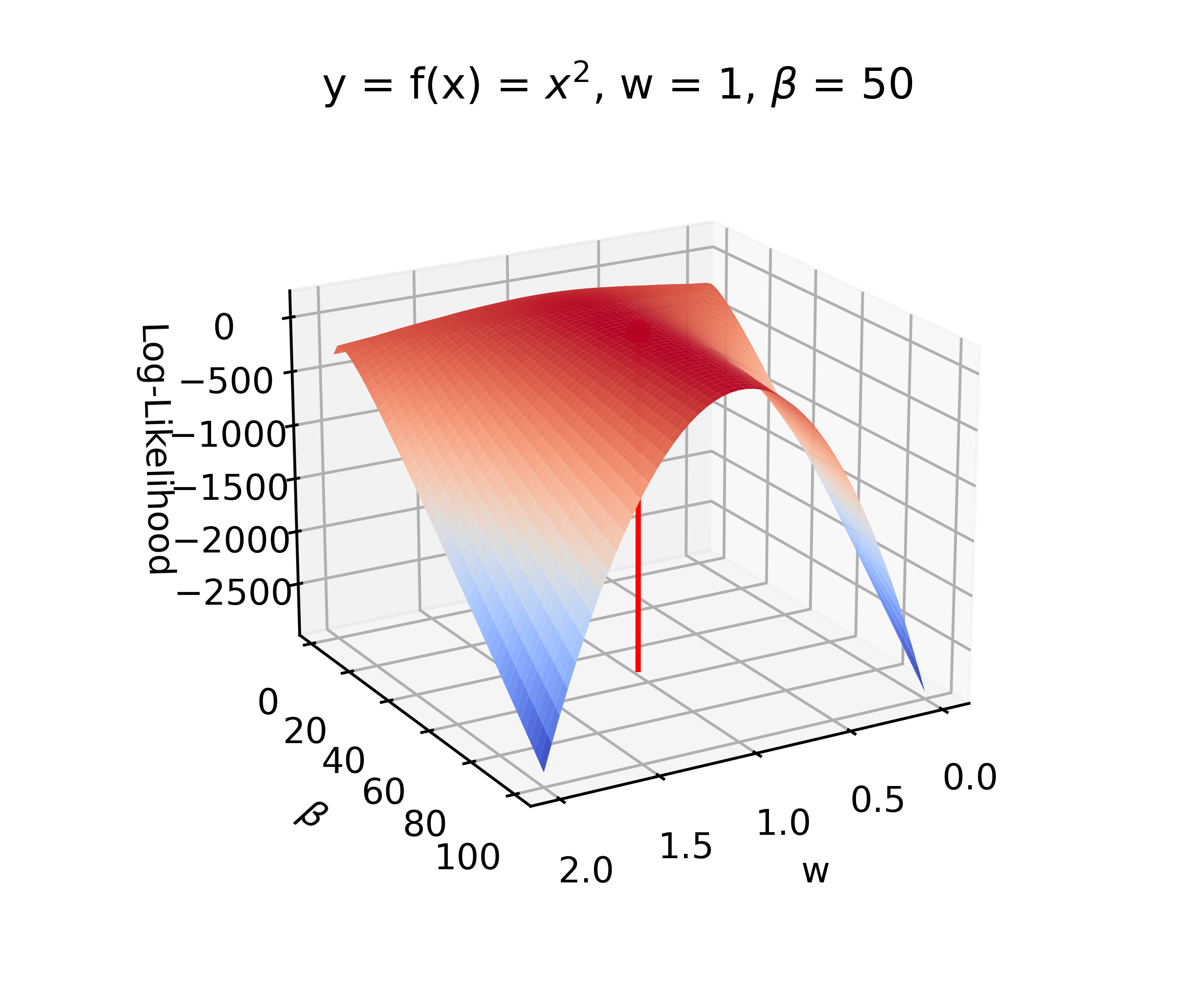
Figure 1: Example of the Maximum-Likelihood approach, with the read line indicating the ML point estimate.
The Prior Distribution
As we have mentioned before, the prior distribution $p(w,\beta)$ can contain any information we have on the unknown parameters. In order to perform Bayesian, it is technically possible to choose any mathematical form of the prior PDF. However, given our likelihood function (2), there are is only one specific parametric prior form that will lead to an analytically tractable posterior distribution. This prior PDF is known as a conjugate prior and will lead to the fact that prior and posterior PDF have the same functional form. For our basic linear regression model this conjugate prior PDF is as follows:
\[p(w,\beta) = p(w|\beta)p(\beta),\]where
\[p(w|\beta)=\mathcal{N}(w|\mu_0,(\beta \tau_0)^{-1})\] \[p(\beta)=\mathcal{Ga}(\beta|a_0,b_0)\]In words, $w$ follows a Normal distribution with mean of $\mu_0$ and a variance conditional on the value of $\tau_0$ and $\beta$, where $\beta$ itself is an unknown parameter that follows a Gamma distribution with shape $a_0$ and rate $b_0$. The exact derivation of this relationship can be found in the Wikipedia entry.
The Posterior Distribution
Having chosen a conjugate prior $p(w,\beta)$ (7)-(9) to our likelihood, the posterior distribution takes the following form:
\[p(w,\beta|\mathcal{D}) = \mathcal{N}(w|\mu_n,(\beta \tau_n)^{-1})\mathcal{Ga}(\beta|a_n,b_n),\]where the hyperparameters of the Normal distribution are calculated by
\[\mu_n=\frac{\tau_0\mu_0+f(x)^Ty}{f(x)^Tf(x)+\tau_0},\] \[\tau_n=f(x)^Tf(x)+\tau_0,\]and the hyperparameters of the Gamma distribution are calculated by
\[a_n = a_0+\frac{N}{2},\] \[b_n = b_0+\frac{1}{2}\left(y^Ty+\mu_0^2\tau_0-\mu_n^2\tau_n\right)\]The details of this derivation can again be found in the Wikipedia entry.
Having calculated the joint posterior density $p(w,\beta|\mathcal{D})$, it can be useful to know the marginal posterior densities over $w$ and $\beta$. For $\beta$ this is very straightforward and we have:
\[p(\beta|\mathcal{D})=\int_{-\infty}^{\infty}p(w,\beta|\mathcal{D})dw=\int_{-\infty}^{\infty}\mathcal{N}(w|\mu_n,(\beta \tau_n)^{-1})\mathcal{Ga}(\beta|a_n,b_n)dw=\mathcal{Ga}(\beta|a_n,b_n)\]For $w$ the process is a bit more complex and involves the calculation of an complicated integral. Using WolframAlpha we can calculate:
\[p(w|\mathcal{D})=\int_{-\infty}^{\infty}p(w,\beta|\mathcal{D})d\beta=\int_{-\infty}^{\infty}\mathcal{N}(w|\mu_n,(\beta \tau_n)^{-1})\mathcal{Ga}(\beta|a_n,b_n)d\beta=C\cdot\Gamma(A+1)B^{(-A-1)}\]with:
\[A=a_n-0.5\] \[B=\frac{\tau_n}{2}(w-\mu_n)^2+b_n\] \[C=\sqrt\frac{\tau_n}{2\pi}\frac{b_n^{a_n}}{\Gamma(a_n)}\]An example of the prior and posterior distributions is given in the following Figure.
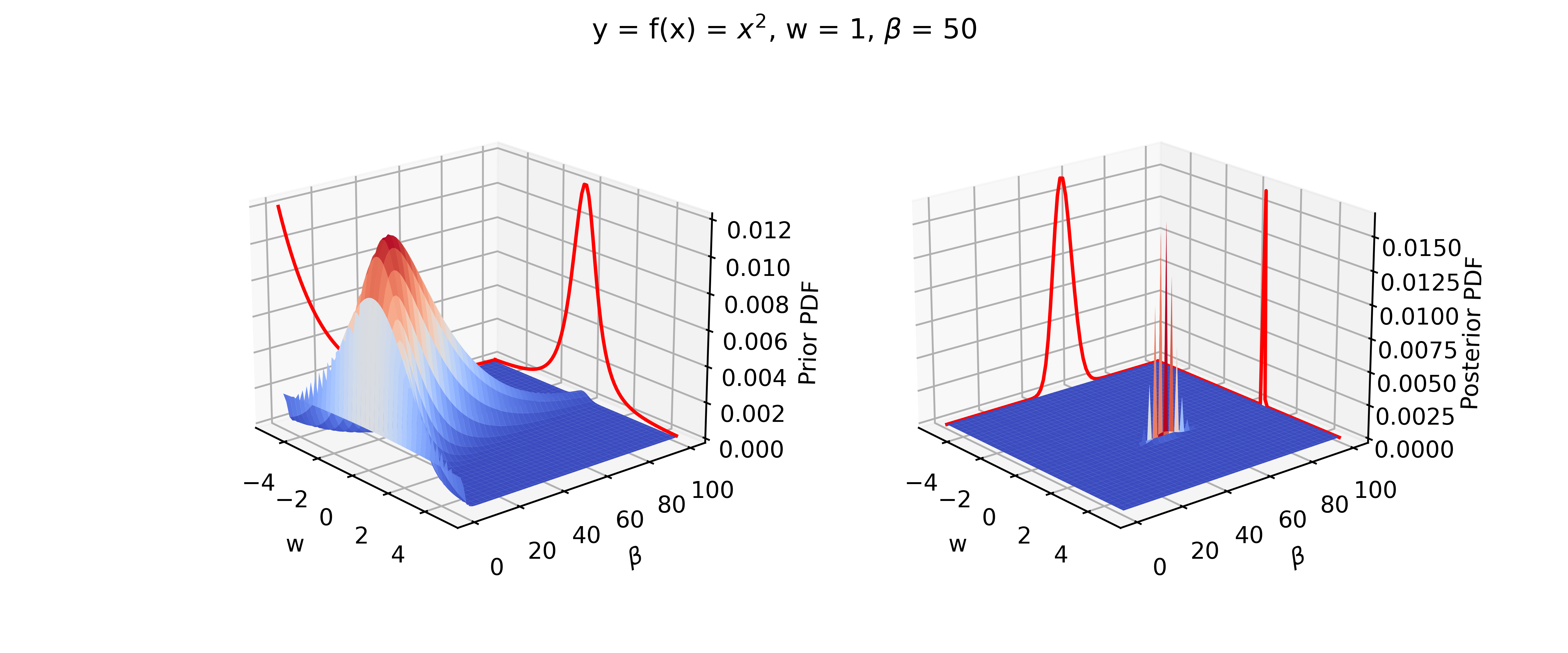
Figure 2: Comparison between prior and posterior distributions. In the right plot, the true value is given in black and the posterior mean in given in red.
Marginal Likelihood
The last thing we can do in this section is to calculate to marginal likelihood defined by:
\[P(\mathcal{D})=\int L(\mathcal{D}|w,\beta)p(w,\beta) dw d\beta\]Again this can be done analytically and it is quite common to calculate the log marginal likelihood:
\[\log P(\mathcal{D})=-\frac{N}{2}\log 2\pi + \frac{1}{2}\log\frac{\tau_0}{\tau_n} + a_0\log b_0 - a_n\log b_n + \log\Gamma(a_n) - \log\Gamma(a_0)\]The marginal likelihood captures in a single number how well our model explains the observations. This number by itself has no meaning, it only becomes interpretable in comparison to other models.
Part 2: Variational Bayesian Approach