Approximate Bayesian Inference using Variational Bayesian Analysis
In variational Bayesian (VB) analysis, the posterior distribution over unknown parameters is approximated by assuming it has certain properties such as factorising in a specific way or taking a specific parametric form. Alongside the approximation of the posterior, the VB method also provides an estimation of the marginal likelihood.
Recap
Before we can begin, we need establish some foundations with respect to the calculations of expectations. The expectation of a function $f(x)$ with respect to some PDF $p(x)$ is expressed as follows:
\[\mathbb{E}[f(x)]_{p(x)}=\int f(x)p(x)dx\]In words, the expectation gives us the expected value of $f(x)$ if we assume that the random variable $x$ follows the PDF $p(x)$. A simple example is the expectation of random variable $x$ that follows a Normal distribution:
\[\mathbb{E}[x]_{\mathcal{N}(x|\mu,\tau^{-1})}=\int x\mathcal{N}(x|\mu,\tau^{-1})dx=\mu\]In words, we expect a random variable $x$ to take the value of the mean $\mu$ if $x$ follows a Normal distribution. As we have seen before, the expectation of a Gamma distribution is:
\[\mathbb{E}[x]_{\mathcal{Ga}(x|a,b)}=\int x\mathcal{Ga}(x|a,b)dx=\frac{a}{b}\]A few more expectations that we will need to know are:
\[\mathbb{E}[x^2]_{\mathcal{N}(x|\mu,\tau^{-1})}=\mu^2+\frac{1}{\tau},\] \[\mathbb{E}[\log x]_{\mathcal{Ga}(x|a,b)}=\psi(a)-\log b,\]where $\psi(\cdot)$ is the Digamma function
The Variational Bayes Approach
We start by introducing the PDF $q(w,\beta)$ which we will use an approximation to the true posterior distribution $p(w,\beta|\mathcal{D})$. Next, we calculate the Kullback-Leibler divergence, between the true and approximated distributions:
\[D_{KL}(q(w,\beta)||p(w,\beta|\mathcal{D}))=\int q(w,\beta)\log\frac{q(w,\beta)}{p(w,\beta|\mathcal{D})}dwd\beta\]The Kullback-Leibler divergence has been introduced in the context of information theory. However, for its use in the VB approach, it has three properties we care about: (1) it is never negative, (2) it is zero if the two distributions are identical and (3) it provides a measure for the similarity between two distributions. Substituting Bayes’ rule for the posterior distribution we get:
\[\begin{aligned} D_{KL}(q(w,\beta)||p(w,\beta|\mathcal{D})) &=\int q(w,\beta)\log\frac{q(w,\beta)P(\mathcal{D})}{L(\mathcal{D}|w,\beta)p(w,\beta)}dwd\beta\\ &=\int q(w,\beta) \left[\log q(w,\beta) + \log P(\mathcal{D}) - \log L(\mathcal{D}|w,\beta) - \log p(w,\beta)\right]dwd\beta\\ &= \mathbb{E}\left[\log q(w,\beta) + \log P(\mathcal{D}) - \log L(\mathcal{D}|w,\beta) - \log p(w,\beta)\right]_{q(w,\beta)}\\ &= \mathbb{E}\left[\log q(w,\beta) - \log L(\mathcal{D}|w,\beta) - \log p(w,\beta)\right]_{q(w,\beta)} + \log P(\mathcal{D})\\ \end{aligned}\]In the last step, we have pulled out the log marginal likelihood from the expectation as it is independent from $w$ and $\beta$. Introducing the Free Energy $\mathcal{F}$ and doing some rearranging we get:
\[\underbrace{\mathbb{E}\left[\log p(w,\beta) + \log L(\mathcal{D}|w,\beta) - \log q(w,\beta)\right]_{q(w,\beta)}}_{\mathcal{F}} = \log P(\mathcal{D}) - D_{KL}(q(w,\beta)||p(w,\beta|\mathcal{D}))\]Now we can see that the Free Energy can be considered a lower bound on the marginal likelihood, in the sense that if the posterior $p(w,\beta|\mathcal{D})$ and approximated distribution $q(w,\beta)$ are identical, then $D_{KL}=0$, which in turn leads to $\mathcal{F}=\log P(\mathcal{D})$. Another interpretation of the expression is that maximising the Free Energy with respect to $q$ minimises the Kullback-Leibler divergence $D_{KL}$. As a result, the Free Energy maximisation provides us with an approximation of the true posterior distribution through $q$ and simultaneously an lower bound on the model evidence through the Free Energy. This is one of the main advantages of the VB method.
Free Energy Maximisation
Maximising the Free Energy (which is a functional) with respect to $q$ is a problem that can be solved using the Variational Calculus, thereby giving the whole method its name. In short, variational calculus gives the tools to optimise functionals (a function that takes another function as input) with respect to some function.
Returning to our problem at hand, we need to introduce the fist approximation of the distribution $q$ in order to maximise the Free Energy. Here, we say that the joint distribution of our unknown parameters can be factorised, i.e.
\[q(w,\beta) = q(w)q(\beta)\]This is known as the mean-field approximation and assumes that there is no conditional dependency between the unknown parameters. The next step is to maximise the Free energy with the individual components of $q$. For that we set
\[\frac{\partial \mathcal{F}}{\partial q(w)}=0\] \[\frac{\partial \mathcal{F}}{\partial q(\beta)}=0\]and solve for $q(w)$ and $q(\beta)$, respectively. This solution is fairly complex and we advise the curious reader to this link, where the steps for the general case are explained. However, an understanding of these steps is not required to follow the rest of this tutorial, or indeed the VB approach, so we will just show the solution. The two densities $q^{}(w)$ and $q^{}(\beta)$ that maximise the Free energy can be calculated as follows:
\[\log q^*(w) = \mathbb{E}[\log L(\mathcal{D}|w,\beta)+\log p(w) + \log p(\beta)]_{q(\beta)}\] \[\log q^*(\beta) = \mathbb{E}[\log L(\mathcal{D}|w,\beta)+\log p(w) + \log p(\beta)]_{q(w)}\]Examining these two equations we can see that they are not independent, i.e. we need $q(\beta)$ to calculate $q^*(w)$ and vice versa. To get around this issue, the VB method employs an iterative maximisation approach, illustrated in the figure below. This means that we initialise both approximated distributions with their respective priors and iteratively update them, always keeping one component constant. After each iteration step, we recalculate the Free Energy. The process is terminated when the change in Free Energy from one step to the next is below some user defined threshold, typically $10^{-3}$ or lower.
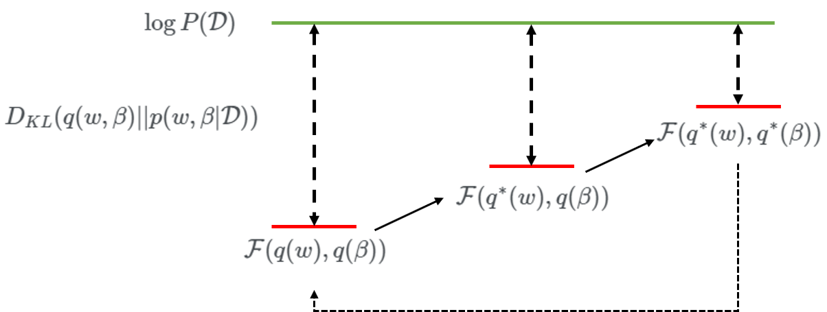
Figure 1: Iterative maximisation of the Free Energy.
Update rules
The previous calculations have been fairly generic as we have not made any assumptions on the parametric forms of the approximate distributions $q(\beta)$ and $q(w)$. In order to proceed, we will assume that $q(w)$ follows a Normal distribution and $q(\beta)$ follows a Gamma distribution, i.e.:
\[q(w,\beta)=q(w)q(\beta)=\mathcal{N}(w|\mu_n,\tau_n^{-1})\mathcal{Ga}(\beta|a_n,b_n)\]Additionally it is assumed that the respective prior distributions have the same parametric form, i.e.
\[p(w,\beta)=p(w)p(\beta)=\mathcal{N}(w|\mu_0,\tau_0^{-1})\mathcal{Ga}(\beta|a_0,b_0)\]With these assumptions, we can see the approximation of prior and posterior in comparison to the “true” distributions, introduced in Part 1 expressions (9)-(11) and (12). Together with the Likelihood function, also introduced in Part 1 expressions (5) - (6), we can now calculate the updated distributions $q^(w)$ and $q^(\beta)$.
Updating $q(w)$
To keep the calculation uncluttered, all terms that are not dependent on the unknown parameter of interest will be collected in a $const$ term. Starting with $q^*(w)$ we have:
\[\begin{aligned} \log q^*(w) &= \mathbb{E}[\log L(\mathcal{D}|w,\beta)+\log p(w) + \log p(\beta)]_{q(\beta)}\\ &=\mathbb{E}[\log L(\mathcal{D}|w,\beta)]_{q(\beta)} + \log p(w) + const\\ \end{aligned}\]Now using the previous definitions of the log-Likelihood and the log Normal distribution from Part 1 we have:
\[\log q^*(w) = -\frac{\mathbb{E}[\beta]_{q(\beta)}}{2} [y^Ty-2wy^Tf(x)+f(x)^Tf(x)w^2] - \frac{\tau_0}{2}[w^2+2w\mu_0-\mu_0^2] + const\]Here, we made use of the fact that we can pull all terms that are not dependent on $\beta$ out from the expectation. Next, we use a technique called completing the square to formulate the expression in terms of a binomial of $w$ so we can extract the hyperparameters of he resulting Normal distribution. For that we collect and sort all terms dependent of $w$ while again summarizing all independent terms in $const$:
\[\log q^*(w) = -\frac{1}{2} [w^2(\frac{a_n}{b_n}f(x)^Tf(x)+\tau_0)- 2w(\frac{a_n}{b_n}y^Tf(x)+\mu_0\tau_0)] + const\]Furthermore we have used the expressions from the beginning of this section. Now we can formulate the binomial:
\[\log q^*(w) = -\frac{\dfrac{a_n}{b_n}f(x)^Tf(x)+\tau_0}{2} \left[w-\frac{\dfrac{a_n}{b_n}y^Tf(x)+\mu_0\tau_0}{\dfrac{a_n}{b_n}f(x)^Tf(x)+\tau_0}\right]^2 + const\]This expression now is in the form of a log Normal distribution and allows us to extract the hyperparameters of the updated Normal distribution as:
\[\tau_n=\dfrac{a_n}{b_n}f(x)^Tf(x)+\tau_0\] \[\mu_n=\dfrac{\dfrac{a_n}{b_n}y^Tf(x)+\mu_0\tau_0}{\tau_n}\]Updating $q(\beta)$
The procedure to derive the update rules for $q(\beta)$ is very similar as before. The main difference is that we want to bring the expression into the form of a log Gamma distribution, which allows us to again extract the updated hyperparameters of the $q(\beta)$. For that we have
\[\begin{aligned} \log q^*(\beta) &= \mathbb{E}[\log L(\mathcal{D}|w,\beta)+\log p(w) + \log p(\beta)]_{q(w)}\\ &= \mathbb{E}[\log L(\mathcal{D}|w,\beta)]_{q(w)} +\log p(w) + const\\ &= \frac{N}{2} \log \beta - \frac{\beta}{2}[-2y^Tf(x)\mathbb{E}[w]_{q(w)}+f(x)^Tf(x)\mathbb{E}[w^2]_{q(w)} + y^Ty] + (a_0-1)\log \beta -b_0 \beta + const\\ &= \log \beta [a_0-1+\frac{N}{2}] - \beta[b_0+\frac{1}{2}[-2y^Tf(x)\mu_n + f(x)^Tf(x)(\mu_n^2+\frac{1}{\tau_n})+y^Ty]]+const \end{aligned}\]Here we have again made use of the expectations with respect to the Normal distribution at the beginning of this part. Now we can extract the hyperparameters of the updated distribution $q(\beta)$:
\[a_n = a_0 + \frac{N}{2}\] \[b_n = b_0+\frac{1}{2}[-2y^Tf(x)\mu_n + f(x)^Tf(x)(\mu_n^2+\frac{1}{\tau_n})+y^Ty]\]Free Energy Decomposition
The last and undoubtedly most complicated thing is to derive the expression for the Free Energy. There are a lot of expressions to formulate but it is essentially just more of the same we have done for the update rules. From expression (7), we have the following expression for the Free Energy.
\[\mathcal{F} = \mathbb{E}\left[\log p(w,\beta) + \log L(\mathcal{D}|w,\beta) - \log q(w,\beta)\right]_{q(w,\beta)},\]which can be expanded as follows (using the previously introduced mean-field approximation):
\[\mathcal{F} = \mathbb{E}\left[\log L(\mathcal{D}|w,\beta) + \log p(w) + \log p(\beta) - \log q(w) - \log q(\beta)\right]_{q(w,\beta)},\]This gives us five terms we can evaluate separately, which is also known as the Free energy decomposition. Starting with the log-likelihood, we have:
\[\begin{aligned} \mathbb{E}[\log L(\mathcal{D}|w,\beta)]_{q(w,\beta)} &= \frac{N}{2}\mathbb{E}\left[\log \frac{\beta}{2\pi}\right]_{q(\beta)} - \frac{1}{2} \mathbb{E}[\beta]_{q(\beta)} \mathbb{E}[y^Ty - 2y^Tf(x)w + f(x)^Tf(x) w^2]_{q(w)}\\ &= \frac{N}{2}\left[\psi(a_n) - \log 2\pi b_n \right] - \frac{a_n}{2b_n}\left[ y^Ty - 2y^Tf(x)\mu_n + f(x)^Tf(x) \left( \mu_n^2 + \frac{1}{\tau_n} \right) \right] \end{aligned}\]Next, the prior distribution $p(w)$:
\[\begin{aligned} \mathbb{E}[\log p(w)]_{q(w)} &= \frac{1}{2} \log \frac{\tau_0}{2\pi} - \frac{\tau_0}{2}\mathbb{E}\left[w^2-2w\mu_0+\mu_0^2\right]_{q(w)}\\ &= \frac{1}{2} \log \frac{\tau_0}{2\pi} - \frac{\tau_0}{2} \left[ (\mu_n^2+\frac{1}{\tau_n}) - 2\mu_0\mu_n + \mu_0^2 \right] \\\end{aligned}\]Next, the prior distribution $p(\beta)$:
\[\begin{aligned} \mathbb{E}[\log p(\beta)]_{q(\beta)} &= a_0 \log b_0 - \log \Gamma(a_0) + (a_0-1)\mathbb{E}[\log \beta]_{q(\beta)} - b_0\mathbb{E}[\beta]_{q(\beta)}\\ &= a_0 \log b_0 - \log \Gamma(a_0) + (a_0-1)\left[ \psi(a_n) - \log b_n \right] - b_0 \frac{a_n}{b_n}\\ \end{aligned}\]Next, the approximated posterior distribution $q(w)$:
\[\begin{aligned} \mathbb{E}[\log q(w)]_{q(w)} &= \frac{1}{2} \log \frac{\tau_n}{2\pi} - \frac{\tau_n}{2}\mathbb{E}\left[w^2-2w\mu_n+\mu_n^2\right]_{q(w)}\\ &= \frac{1}{2} \log \frac{\tau_n}{2\pi} - \frac{\tau_n}{2} \left[ (\mu_n^2+\frac{1}{\tau_n}) - 2\mu_n^2 + \mu_n^2 \right] \\ &= \frac{1}{2} \log \frac{\tau_n}{2\pi} - \frac{1}{2}\end{aligned}\]Lastly, the approximated posterior distribution $q(\beta)$:
\[\begin{aligned} \mathbb{E}[\log q(\beta)]_{q(\beta)} &= a_n \log b_n - \log \Gamma(a_n) + (a_n-1)\mathbb{E}[\log \beta]_{q(\beta)} - b_n\mathbb{E}[\beta]_{q(\beta)}\\ &= a_n \log b_n - \log \Gamma(a_n) + (a_n-1)\left[ \psi(a_n) - \log b_n \right] - a_n\\ \end{aligned}\]This finishes the Free Energy decomposition.
Implementation of the Algorithm
Using pseudocode, the VB algorithm for parameter estimation and Free Energy calculation can be implemented as follows:
# Calculate Prior Free Energy
F(1) = Calculate Free Energy (a0, b0, mu0, tau0)

an = a0
bn = b0

mun = mu0
taun = tau0

k=2
dFtol = 1e-3

# Free Energy maximisation loop
while dF > dFtol
    Calculate an, bn        # Update q(beta)
    Calculate mun, taun     # Update q(w)

    # Calculate Free Energy
    F(k) = Calculate Free Energy (an, bn, mun, taun)

    dF = F(k) - F(k-1)
    k=k+1
end
Example results
Coming back to our example model we get the following results.
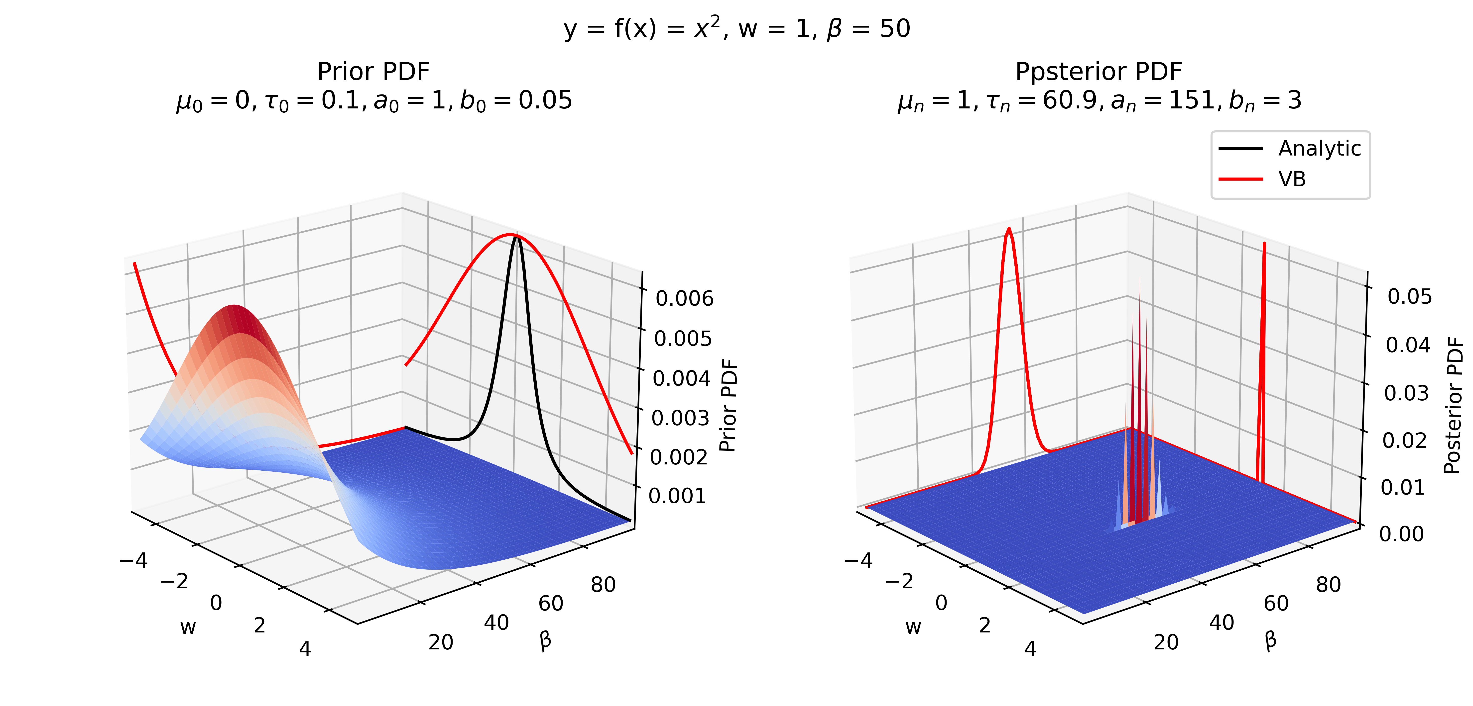
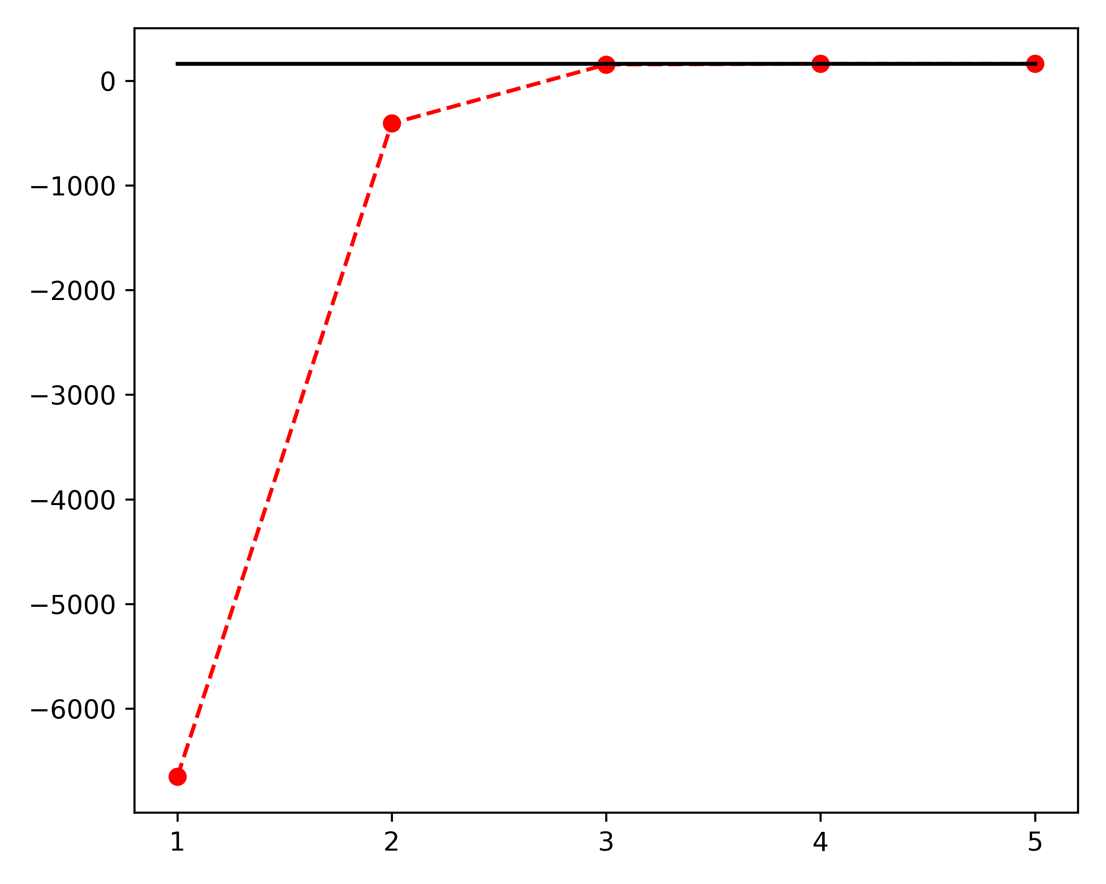
We can see that the prior distributions differ quite significantly as a result of the mean-field approximation. However, the posterior results are very similar, showing the utility of the approximation. The iterative maximisation of the Free Energy and approximation to the true log marginal likelihood is shown in the following figure.